PHASER: Phaser Modules Discrete Chaos

Modules: Discrete Chaos

Chapter 2: Stability of Two-Dimensional Maps

Section 4.4: Second-Order Difference Equations

Example 4.4:
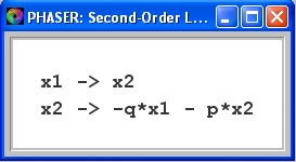
Second-order difference equations can be solved numerically using Phaser. However, before they can be entered into Phaser, they must be converted to a pair of first-order difference equations. Consider, for example, the linear second-order difference equation x(t+2) + p x(t+1) + q x(t) = 0. Using the new variables x(t) = x1 and x(t+1) = x2, this second-order equation is equivalent to the linear system of first-order equations:

(1)

where p and q are parameters.

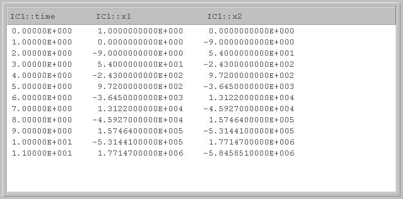
Figure 4.4.1. Solution of Eq.(1) satisfying the initial conditions x1 = 1, x2 = 0, for the parameter values p = 6, q = 9.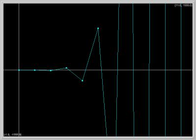

Figure 4.4.2. Graph of the solution in the (x1, t) plane from the previous figure.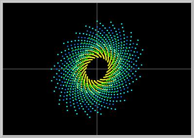

Figure 4.4.3. Phase portrait of Eq.(1) in the (x1, x2)-plane for p = -0.4, q = 0.995. The origin is an asymptotically stable fixed point.

Activities:

Click on the first picture to load it into your local copy of Phaser. Verify that the values of x1(t) agree with the formula x1(t) = (-3)^t(1 - t).
Click on the third picture to load it into your local copy of Phaser. Change the parameter q = 1. (PhaserTip: Changing Parameters) Clear and Go. Do you notice any qualitative change in the picture?
Change the parameter q = 1.01. Clear and Go. Do you notice any qualitative change in the picture?

[ Previous Section | Next Section | Main Index | Phaser Tips ]