PHASER: Module: Leibnitz's Pocket Watch ODE

Trajectory of a pocket watch - Tractrix

Highlights:

Leibniz Historical: "The distinguished Parisian physician Claude Perrault, equally famous for his work in mechanics and in architecture, well known for his edition of Vitruvius, and in his lifetime an important member of the Royal French Academy of Sciences, proposed this problem to me and to many others before me, readily admitting that he had not been able to solve it ..." (Leibniz 1693)

Mathematical: The trajectory of a pocket watch pulled horizontally from its chain is the curve tractrix.

Prerequisites:

Separation of Variables

Equation:

dy/dx = -y / (a² - y²)^1/2

Variables:
x : Horizontal coordinate of the position of the pocket watch
y : Vertical coordinate of the position of the pocket watch

Parameter:
a : Length of pocket watch chain

Discussion:

Take a pocket watch ("horologio portabili suae thecae argenteae") with a chain and put it on a table top. Pull the end of the chain along a line. What is the trajectory of the watch?

In the presence of moderate friction on the surface of the table, it is reasonable to assume that the chain will be tangent to the trajectory of the pocket watch. Let us denote the trajectory with the function y(x). As it can readily be seen in the Figure on the left, the slope of the chain dy/dx is -y/b, where b = (a² - y²)^1/2. Therefore, the trajectory y(x) satisfies the Leibniz ODE given above.

Geometrically, this problem can be recast as follows: find a curve with the property that at each point on the curve, the tangent line segment between the point of tangency and the x-axis is of constant length a. Such a curve is called the tractrix or equitangential curve. It was first studied by Huygens in 1692 who gave its name - tractrix.

Dynamics:

The formula for the path of the pocket watch, as Leibniz said, is complicated. Here it is:

x - x₀ = - (a² - y²)^1/2 - a log(y) + a log (a + (a² - y²)^1/2) + (a² - y₀²)^1/2 + a log(y₀) - a log (a + (a² - y₀²)^1/2)

This formula is the solution of the differential equation satisfying the initial condition y(x₀) = y₀, which is given implicitly.

Rest assured that the derivation of this formula will be forthcoming. Despite this formula, however, the question remains: what is the trajectory of the pocket watch look like? One can, of course, attempt to plot the graph of this function using a function plotter. Note, however, that this is an implicit formula which gives an expression for x in terms of y, rather than the other way around. So, if you plot x as a function of y, make sure to tilt your head 90^o.

Phaser simulation: To see a trajectory of the pocket watch, let us turn to Phaser, rather than a function plotter. A numerical solution of an initial-value problem for the Leibniz ODE is plotted in Figure 1. below.

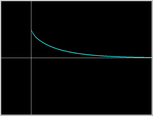
Figure 1. A trajectory of Leibniz's pocket watch - tractrix.
Click on the picture to load it into your local Phaser.

Historical considerations aside, the qualitative dynamics of this model is rather simple. y = 0 is an asymptotically stable equilibrium point. All solutions starting near the equilibrium point eventually approaches the equilibrium. Note, however, that the equation is defined for only initial data |y(x₀)| < a.

Mathematical results:

The solutions of Leibniz ODE can be obtained using the Method of Separation of Variables. Indeed, the discovery of this powerful method is often attributed to Leibniz. One of the required integrals for the solution is somewhat difficult to evaluate. The details of this integration using a trigonometric substitution is available in a PDF file.

The surface of revolution generated by revolving the tractrix about its asymptote, the x-axis, is called the pseudo-sphere. The pseudo-sphere has constant negative Gaussian curvature, this is in contrast to the standard sphere which has constant positive Gaussian curvature. A triangle on a pseudo-sphere has total interior angles less than 180^o, while a triangle on a sphere has total angles greater than 180^o. The pseudo-sphere was one of first models of non-Euclidean geometry and was investigated by Beltrami in 1868.

Suggested Explorations:

Build an apparatus: tape a pencil on a block of wood and attach a piece of string to the block. Drag the block while pulling the string along a line. Does the curve traced by the pencil resemble the computer generated trajectory?
What happens if initial data y₀ is bigger than a?
Evaluate the integral resulting from separation of variables, as Leibniz did, using the substitution
(a² - y²)^1/2 = v, a² - y² = v², -y dy = v dv.
In differential geometry, a parameterization of the tractrix, for a = 1, is given by the equations
x(t) = t - tanh(t), y(t) = sech(t).
Show that this parameterized curve satisfies the differential equation. Hint: compute (dy/dt)/(dx/dt) and use hyperbolic identities.
Load the Phaser Project in Figures 1. Click the left mouse button at several locations to mark additional initial conditions. Now click the Go button to see that all solutions (provided that y₀ < a) converge to the equilibrium solution y(x) = 0. Draw the phase portrait of the differential equation.
Linearize the differential equation about the equilibrium point y = 0 and verify, using the Linearization Theorem that the equilibrium point is asymptotically stable.

Related modules:

None.

References:

HAIRER, E. [1996]. Analysis by Its History. Springer-Verlag, New York.

LEIBNIZ, G.W. [1693]. "Supplementum geometriae dimensoriae, seu generalissima omnium tetragonismorum effectio per motum: similiterque multiplex constructio linea ex data tangentium conditione," Acta Eruditorum, 12, 385-392.

MILLMAN, R. and PARKER, G. [1974]. Elements of Differential Geometry. Prentice-Hall, Inc.

O'CONNOR, J.J. and ROBERTSON, E.F. Gottfried Wilhelm von Leibniz. http://www-gap.dcs.st-and.ac.uk/~history/Mathematicians/Leibniz.html

RICKEY, V.F. [1995]. "My favorite ways of using history in teaching calculus," Learn from the masters!, edited by F. Swetz. Mathematical Association of America.

Feedback:

Please write to us with your comments on this module.