A pioneering model of a density-dependent population

Highlights:

Ecological: "Plotting net reproduction (reproductive potential of the adults obtained) against the density of stock which produced them, for a number of fish and invertebrate populations, gives a domed curve whose apex lies above the line representing replacement reproduction. At stock densities beyond the apex, reproduction declines either gradually or abruptly. This decline gives a population a tendency to oscillate in numbers; however, the oscillations are damped, not permanent, unless reproduction decreases quite rapidly and there is not too much mixing of generations in the breeding population. Removal of part of the adult stock reduces the amplitude of oscillations that may be in progress and, up to a point, increases reproduction." --- Ricker [1954].

Mathematical: A specific example of such a model reproduction curve, framed in terms of a 1D difference equation, is the Ricker MAP. For certain ranges of the growth rate, this map indeed exhibits stable and unstable oscillations. Moreover, as the growth rate is increased further, the map undergoes a sequence of period-doubling bifurcations, eventually leading to chaotic dynamics.

Prerequisites:

Fixed Points of 1D MAPs, Period-doubling bifurcations of 1D MAPs.

Equation:

N_n+1 = N_n e ^{r ( 1 - N_n / K )}

Variables
N_n : Density of population at generation n
N_n+1 : Density of population at generation n+1

Parameters
K : Carrying capacity
r : Growth rate of the population

Discussion:

Moran [1950] in his illuminating paper on the various ways in which mathematics is applied to biological problems writes:

"Consider now the problem of explaining why cyclical behaviour does occur in animal populations. All or nearly all the mathematical theories constructed to account for these observations depend on the interaction between two or more populations of animals and undoubtly this must play a major part in most observed cycles. In the present paper we shall consider that may happen in a single population independently of changes in other populations."

If we let N(t) denote the size of a single population changing (differentiably) as a function of time t, then the change of the population size over time can usually be modeled using an appropriate 1D (scalar) autonomous differential equation of the form dN/dt = F (N). Solutions of any scalar autonomous differential equation are monotone function of time; they cannot oscillate in time. For example, the famous logistic differential equation dN/dt = r N (1 - N/K) has the following typical solutions: solutions move monotonically towards the carrying capacity without oscillations, as seen in Figure 1.

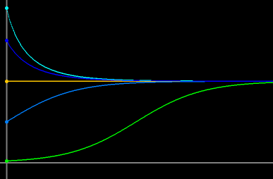
Figure 1. Typical solutions of Logistic Differential Equation.
They approach the carrying capacity monotonically, without oscillations.
Click on the image to load it into your local Phaser.

In modeling certain populations, it may be more appropriate to use difference equations instead of differential equations. For example, in seasonally breeding populations whose generations do not overlap, it suffices to keep track of the population once every generation. In such a situation, one can describe the change in the population with a difference equation of the form

N_n+1 = f ( N_n )

where N_n is the population size at the n-th generation and the function f is the reproduction function. The graph of f when plotted on the (N_n, N_n+1) plane is called the reproduction curve. In his seminal paper, Ricker [1954] writes:

"Towards a theory of recruitment: The justification for using any reproductive curve must in the long run come from observations. However it would be most useful, if it were possible, to formulate some general theory of reproduction which might lead to a standard type of reproduction curve applicable in majority of situations."

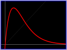
Indeed, the specific form of the reproductive curve
f( N_n ) = N_n e ^{r ( 1 - N_n / K )}
we use here is suggested by Ricker, based on his careful examination of "a number of fish and invertebrate populations." A detailed construction of this model, with the standing biological assumptions, is given in Ricker [1954]. A modified, and perhaps simpler, derivation is in Greenwell and Ng [1984].

Dynamics:

The dynamics of the Ricker MAP undergo complicated variations as the parameter r is varied. However, the basic ecologically relevant features can be readily uncovered through Phaser simulations as we demonstrate below.

Phaser simulations:

• Figure 2: Reproduction curves: A Gallery of reproduction curves as the growth rate r is increased, while the carrying capacity K is held fixed.

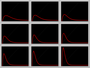
Figure 2. A Gallery of reproduction curves.
Click on the image to load it into your local Phaser.
To see a sequence of reproduction curves, hit the
"Slideshow" button on the button bar of the spawned Gallery, and Play.

• Figure 3a: Stable oscillations: For r > 0, the map has a fixed point with positive coordinate equal to the carrying capacity K. For 0 < r ≤ 2, the fixed point is asymptotically stable and the approach to this fixed point is oscillatory.

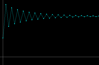
Figure 3a. For r = 1.9, stable oscillations of the population size as a function of generations.

• Figure 3b: Stair-step diagram: It is often more illuminating to follow the solutions of a 1D difference equation by plotting the next generation as a function of the current generation. The intersections of the reproduction curve with the 45-degree line correspond to fixed points. Here, the solution in Figure 3a viewed in a stair-step diagram.

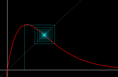
Figure 3b. For r = 1.9, the asymptotically stable fixed point viewed in a stair-step diagram.

• Figure 4: Period doublings: As the parameter r is increased beyond 2, the positive fixed point becomes unstable and gives rise to an asymptotically stable periodic orbit of period 2. As the parameter is increased further, the period 2 orbit becomes unstable and gives rise to a period 4 orbit, and so on.

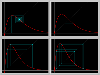
Figure 4. Period doubling bifurcations viewed in stair-step diagrams.
Fixed point -> Period 2 -> Period 4 -> Period 8.

• Figure 5: Bifurcation diagram: As the parameter is increased further, the period doubling bifurcations happen at a geometric rate leading to chaotic dynamics at about r = 2.6924... . An effective way to follow these bifurcations, and more, is to generate a Bifurcation Diagram as seen below.

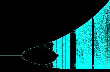
Figure 5. Bifurcation diagram as the as parameter r is varied.

Experimental data:

In his seminal paper, Ricker [1954] remarks that "the justification for using any reproduction curve must in the long run come from observation." Indeed, he constructs reproduction curves of half dozen fish species, fruit fly (Drosophila melanogaster), and water-flee (Daphnia magna) from experimental data before ariving at the theoretical model under consideration in this module. One noteworthy example is the reproduction curves of pink salmon (Oncorhynchus gorbuscha) from data (Figures 19-20) and fitting the data to the model (Table VIII).

In Murphy [1967], "The population parmaters of the Pacific sardine (Sardinops Caerulea) are estimated from growth, mortality, and fecundity data, together with increase per generation estimated by fitting the Ricker equation." Also, a modification of the deterministic Ricker MAP with a uniformly distributed random variable to account for random environmental factors.

Block and Kocak [2005] analyze the salmon count data from six dams along the Columbia and Snake rivers. They estimate the parameters in the Ricker MAP from this data using elementary statistical methods.

Remarks:

Here is what The Great Canadian Scientists (GCS) Research Society says about Ricker on its Web site:

"Canada's Greatest Fisheries Biologist: Inventor of the Ricker Curve for describing fish population dynamics. ... The Ricker Curve is still used all over the world to determine average maximum catches for regional fisheries."

This model is historically one of the most significant uses of difference equations (MAPs) in modeling density-dependent populations with non-overlapping generations. Although it is a theoretical model, it is designed to capture the common features of many experimentally determined reproduction curves. It succeeds in providing a quantitative possibility of oscillations that are observed in fish populations. Of course, the model has obvious shortcomings: as it does not reflect the outside influences on the salmon populations, such as dams or other man-made impediments, pollution, or random environmental variations. Still, every student of quantitative ecology should be aware of the Ricker MAP.

Suggested Explorations:

1. Dependence on K: Load the Phaser Gallery in Figure 2. Investigate the dependence of the reproduction curve on the parameter K while r is fixed.
2. Fixed points: Verify that N = 0 and N = K are the only fixed points of the Ricker MAP when r > 0. Using linearization, investigate the stability types of these fixed points for all parameter values r > 0 and K > 0. Discuss the ecological significance of your findings. What happens to the map, and the fixed points, when r = 0?
3. Asymptotically stable?: For r = 2, the derivative of the Ricker MAP at the positive fixed is -1 (non-hyperbolic fixed point); hence the linearization is inconclusive. Load Figure 3b into your local Phaser and verify that the fixed point is asymptotically stable for r = 2. Rate of approach to a nonhyperbolic fixed point can be painfully slow, so increase Time substantially to observe asymptotic stability.
4. Bounds: Since the reproduction curve has a maximum, the population is bounded above; find this maximum value. Aside from some possible initial transient values, the minimum population value happens to be the generation immediately following the maximum value; find this minimum value.
5. Global attraction: The positive fixed point is globally attractive for r ≤ 2. If you are familiar with Lyapunov functions for difference equations you should consult May [1974] and Goh [1977]. In any case, you should try many initial conditions to test this conclusion numerically.
6. Multiple attractors?: Compute the bifurcation diagram with several initial conditions in case there are multiple coexisting attractors.
7. Period 3: There is an attacting periodic orbit of period three for r = 3.12. Can you find another value of r for which there is a period 3 orbit? (Hint: examine the gaps in the bifurcation diagram.)

Related modules:

Beddington-Free-Lawton MAP: Stabilizing Nicholson-Bailey with host density dependence.

References:

BLOCK, C. and KOCAK, H. [2005]. "Will the salmon obey Ricker?," (pdf). A student-authored Phaser Module at www.phaser.com

FISHER, M.E., GOH, B.S., and VINCENT, T.L. [1979]. "Some stability conditions for discrete-time single species models," Bulletin of Mathematical Biology, 41, 861-875.

GOH, B.S. [1977]. "Stability in a Stock Recruitment Model of an Exploited Fishery," Math. Biosci. 33, 359–372.

GREENWELL, R.N. and NG, H.K. [1984]. "The Ricker salmon model," The UMAP Journal, 5, 339-359.

HASTINGS, A. [1997]. Population Biology: Concepts and Models. Springer-Verlag New York, Inc.

MAY, R.M. [1974]. "Biological Populations with Non-Overlapping Generations: Stable Points, Stable Cycles and Chaos," Science, 186, 645–647.

MAY, R.M. and OSTER, G.F. [1976]. "Bifurcations and dynamic complexity in simple biological models," The American Naturalist, 110, 573-599.

MORAN, P.A.P. [1950]. "Some remarks on animal population dynamics," Biometrics, 6, 250-258.

MURPHY, G.I. [1967]. "Vital Statistics of the Pacific Sardine (Sardinops Caerulea) and the Population Consequences," Ecology, 48, 731-736. JSTOR URL

RICKER, W.E. [1954]. "Stock and recruitment," J. Fisheries Res. Board Can., 11, 559-623.

Feedback:

Please write to us with your comments about this module.