A discrete population model of delayed regulation
Highlights:
 Ecological:
"In nature,
the events are not continuous, but dependent on a seasonal cycle
which probably enhances oscillations generated by the purely internal
demographic factors. It is quite possible that phenomena of this sort,
which, in effect, involve the operation, with a time lag, of population
density on net rate of increase, play a part in generating the well-known
cyclic changes in the populations of field mice."
---
Hutchinson [1948].
Ecological:
"In nature,
the events are not continuous, but dependent on a seasonal cycle
which probably enhances oscillations generated by the purely internal
demographic factors. It is quite possible that phenomena of this sort,
which, in effect, involve the operation, with a time lag, of population
density on net rate of increase, play a part in generating the well-known
cyclic changes in the populations of field mice."
---
Hutchinson [1948].
Mathematical: "... a fixed point bifurcates into a smooth invariant circle which somehow transforms itself into a strange attractor as the parameter is increased. Our object is to elucidate the mechanism by which this transformation occurs. We first attempted to pin down the precise parameter value at which the circle loses its integrity. To our surprise, we found that there is no unique parameter value which divides nice behavior from strange behavior. There are parameter intervals for which the attractor appears to be a smooth invariant circle interspersed among parameter intervals for which the attractor appears to be strange. The more precision we used in our investigation, the more interspersed intervals we found. We tried to catalog various types of behavior, but could find no simple patterns." --- Aronson et al. (1982)
Prerequisites:
Fixed Points of 2D MAPs, Neimark-Sacker bifurcation of 2D MAPs.
Equation:
Nn+1 = a Nn( 1 - Nn-1)
Variables:
Nn-1 : Density of population at generation n-1
Nn : Density of population at generation n
Nn+1 : Density of population at generation n+1
Parameter:
a : Intrinsic growth rate of the population
Discussion:
Hutchinson [1948] appears to be the first ecologist to investigate the role of explicit delays in ecological models. He considered the differential-delay logistic equation dx(t)/dt = x(t)(a - b x(t-T)) with delay T. Here, in constrast with the usual logistic differential equation, it is assumed that the amount of resources available at time t will depend on the density of the species at an earlier time by a delay of T. Since Huthinson's work, delay differential equations have occupied the attention of a great number of ecologists as well mathematicians. For various models of such equations in ecology, see, for example, GOPALSAMY [1982].In this Module, we will examine a discrete analog of Huthinson's equation that was introduced by MAYNARD SMITH [1968] with the following introduction:
Delayed Regulation: It is possible that the reproductive rate R may depend not only on the population density at the time, but on the population density in the past. For example, the reproduction of a herbivorous species will depend on the vegetation, which may in turn depend on how much of the vegetation was eaten by herbivores in the pervious year. To gain some idea of the effect of such a delay in the effects of population density on its own increase, a much over-simplified example will be considered. It will be assumed that R depends only only on the population density in the previous year, and not on the immediate density nor on the density in still earlier years.
In modeling seasonally breeding populations whose generations do not overlap, it suffices to keep track of the population once every generation. In such a situation, one can describe the change in the population with a difference equation of the form
Nn+1 = R Nn
where Nn is the population size at the n-th generation and R is the reproductive rate. Now, following MAYNARD SMITH, we assumes the form
R = a(1 - Nn-1)
for reproductive rate to arrive at the difference equation
Nn+1 = a Nn ( 1 - Nn-1 ) .
This equation is almost like the famous logistic map except that the factor regulating the population growth contains a time delay of one generation. To follow the fate of a population, the density of the first two generations must be known. Here the parameter a is called the intrinsic growth rate. Below, we will examine the dynamics of this model as we vary the value of this important parameter.
Converting Second-Order MAP to First Order: For the purposes of mathematical analysis and computer simulations, it is desireable to convert the second-order difference equation
Nn+1 = a Nn ( 1 - Nn-1 ) ,
where the right-hand side is a function of the two previous generations (iterates), to an equivalent pair of first-order difference equations. To this end, we introduce two new variables (x1) and (x2), and set
(x1)n = Nn-1
(x2)n = Nn .
Now, the difference equations for x1 and x2 become the following pair
(x1)n+1 = (x2)n
(x2)n+1 = a (x2)n
(1 - (x1)n) .
of first-order difference equations. To avoid the over-abundant subscripts, we prefer to write this system of first-order difference equations as the iteration of the MAP
x1 -> x2
x2 -> a x2 (1 - x1) .
These are the equations stored in the MAP Library of Phaser under the name Delayed Logistic MAP. We will this planar MAP for the PHASER simulations below.
Dynamics:
The dynamics of the Delayed Logistic MAP undergo complicated and subtle variations as the parameter a is varied. However, the basic ecologically relevant features can be readily uncovered through Phaser simulations as we demonstrate below.The Delayed Logistic MAP has two fixed points; one at the origin (x1, x2) = (0, 0) and the other at (1-1/a, 1-1/a). When a>1, the second fixed point lies in the first quadrant and thus biologically significant. The eigenvalues of the linearized map (Jacobian) at the origin are 0 and a; thus the origin is asymptotically stable for 0 < a < 1, and unstable for a > 1. The eigenvalues at the other fixed point are 0.5(1 ± (5 - 4a)1/2). For 1 < a < 2, the eigenvalues have moduli less than 1, and thus the fixed point is asymptotically stable. It is the dynamics of this fixed point that we will explore first using PHASER.
Phaser simulations:
- Figure 1: Monotone approach to fixed point: For 1 < a < 1.25, the origin is unstable and the other fixed point in the first quadrant is asymptotically stable with real eigenvalues. Thus solutions starting near this fixed point approach it monotonically.
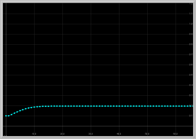
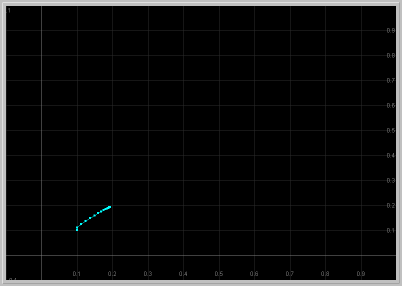
Figure 1. a = 1.24: x1 vs. t
and x1 vs. x2 for 60 generations.
The population approaches the fixed point monotonically.
Click on the image to load it into your local Phaser.
- Figure 2: Damped Oscillations: For 1.25 < a < 2, the fixed point in the first quadrant is asymptotically stable with complex eigenvalues. Thus solutions starting near this fixed point exhibit damped oscillations as they approach the fixed point.
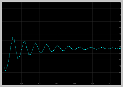
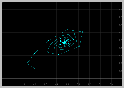
Figure 2. a = 1.9: x1 vs. t
and x1 vs. x2 for 60 generations.
The population approaches the fixed point with damped oscillations.
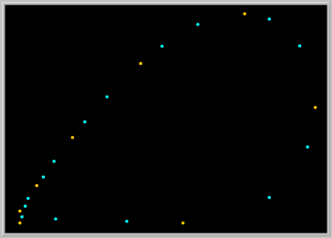
- Figure 3: Sustained Oscillations: For a > 2, the positive fixed point becomes unstable. Now that both fixed points are unstable, where can solutions go? They exhibit sustained oscillations that are periodic or quasi periodic, as seen below.
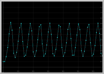
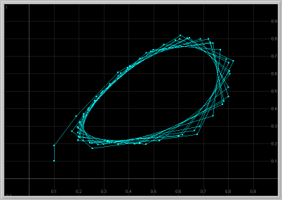
Figure 3. a = 2.1: x1 vs. t
and x1 vs. x2 for 60 generations.
The population exhibits sustained oscillations.
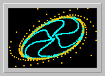
- Figure 4: Poincare-Andoronov-Hopf Bifurcation for Maps: This is the important bifurcation (also called Neimark-Sacker Bifurcation) of a fixed point of a planar map depending on one parameter in the case where the eigenvalues are complex conjugate and of unit moduli. As the eigevalues move off the unit circle, the generic result is that there appears a closed invariant curve--all the iterates of a point on the curve remain on the curve--encircling the fixed point. For a precise statement of this bifurcation, see, for example, HALE and KOCAK [1991], page 473. The Delayed Logistic MAP undergoes Poincare-Andoronov-Hopf Bifurcation as the parameter passes through a = 2. One of the genericity conditions of this theorem is that the eigenvalues not be the first four roots of unity. It is visually evident in Figure 4 that this requirement is indeed fullfilled for the Delayed Logistic MAP.
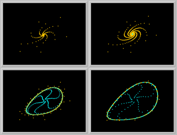
Figure 4. A Gallery of phase portraits as the parameter a is increased
through a = 2.
Click on the image to load it into your local Phaser.
To see the bifurcation in action, hit the
"Slideshow" button on the button bar of the spawned Gallery,
and "Play".
- Figure 5: Coexisting Periodic Attractors: As the parameter a is increased further away from 2, the topology of the invariant curve and the dynamics on it can undergo rapid changes. For example, for a = 2.23444, there are two coexisting asymptotically stable periodic orbits.
- Figure 6: A Strange Attractor: As the parameter a is increased further, the invariant closed curve loses its smoothness and breaks down, giving rise to a strange attractor. Repeated enlargements of portions of the stange attractor reveal a cantor set structure similar to the one in the famous Henon attractor.
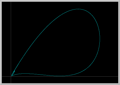
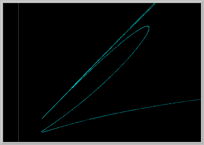
Figure 6. a = 2.265. A strange attractor and enlargement of a piece of it.
- Figure 7: Bifurcation diagram:
As the parameter a is increased further away from
the Poincare-Andronov-Hopf bifurcation, the dependence of the dynamics
of the Delayed Logistic MAP is remarkably intricate.
Indeed, ARONSON et al [1982] who nearly unravel this complexity
(see also POUNDER and ROGERS [1980]), conclude
their seminal paper with the words:
One can see that it is quite difficult to draw a one parameter subfamily through the infinite number of resonance horns without passing many times through regions of relative simplicity interspersed with regions of relative complexity. In one parameter families the transition from simple to complicated behavior is itself quite complicated.
An effective way to follow visible attractors as the parameter a is increased is to generate a Bifurcation Diagram as seen below. Make sure you enlarge various parts of the diagram to explore some of this bewildering complexity.
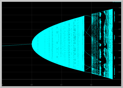
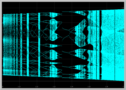
Figure 6. Bifurcation diagram and enlargement of a piece of it
as the parameter a is varied.
Experimental data:
TURCHIN [1990], in his paper titled "Rarity of density dependence or population regulation with lags?", presents convincing experimental evidence for delayed regulation in 14 forest insect populations:Several recent reviews of published life tables concluded that density-dependent regulation is infrequent in insect populations, prompting a vigorous debate among ecologists. Little attention, however, has been directed to one issue: most life-table analyses look only for direct (not-lagged) density dependence. Thus, there is a real danger that populations characterized by delays in regulation will be relegated to a density-independent limbo by an analysis not equipped to recognize such behaviour. I have evaluated the evidence for delayed density dependence in population dynamics of 14 forest insects, and assessed the effect of regulation lags on the likelihood of detecting direct density dependence. Eight cases exhibited clear evidence for delayed density dependence and laginduced oscillations, but direct density dependence was detected in only one of these. This result suggests that traditional analyses will not, in general, detect density-dependent regulation in populations that are characterized by lags and complex dynamic behaviour.As one of his approaches, Turchin uses an extension of the classical Ricker MAP with a lag of one generation. He then demonstrates that, in 8 out of 14 insect populations, the delayed version of the Ricker model results in better fit for the field data then the classical Ricker MAP with no delay. A version of Delayed Ricker MAP is available in the Suggested Explorations below.
Suggested Explorations:
- Fixed points: Verify that the Delayed Logistic MAP has only two fixed points; one at the origin (x1, x2) = (0, 0) and the other at (1-1/a, 1-1/a). Compute that the eigenvalues of the linearized map (Jacobian) at the origin are 0 and a; and the eigenvalues at the other fixed point are 0.5(1 ± (5 - 4a)1/2).
- Global attraction?: As seen in Figure 2b, the positive fixed point is asymptotically stable for a = 1.9. Does this fixed point attract all solutions starting in the first quadrant? Load this figure into your local Phaser and should try many initial conditions to for an answer.
- Asymptotically stable?: For a = 2, the eigenvalues at the positive fixed have moduli 1 (non-hyperbolic fixed point); hence the linearization is inconclusive. Load Figure 2b into your local Phaser and verify that the fixed point is asymptotically stable for the Parameter value a = 2. Rate of approach to a non-hyperbolic fixed point can be painfully slow, so increase Time substantially to observe asymptotic stability.
- Multiple attractors?: Compute the bifurcation diagram with several initial conditions in case there are multiple coexisting attractors.
- Longer delays:
Consider the third-order difference equation
Nn+1 = a Nn ( 1 - Nn-2 ) ,
where the reproductive rate term has delay of two generations. Determine value of the parameter a when the positive fixed point becomes unstable and the system starts exhibiting sustained oscillations. Is the value of a you find smaller or larger than the value of a in the case of delay of one generation? For further information on the effects of longer delays for oscillations, see LEVIN and MAY [1976] or KOT [2001].
- Delayed Ricker MAP:
x1 -> x2
x2 -> x2 exp(r + ax2 + bx1) .
This is a version of delayed Ricker MAP used in TURCHIN [1990]. Click on this delayed_ricker.ppf PHASER project to load it into your local PHASER and investigate its dynamics.
- Delayed Beverton-Holt MAP:
Convert the second-order delayed Beverton-Holt model
Nn+1 = r Nn / ( 1 + [(r - 1)/K] Nn-1 )
to an equivalent pair of first-order equation. Fix K and study the dynamics as a function of r. Can you get damped or sustained oscillations?
Related modules:
Beddington-Free-Lawton MAP: Stabilizing Nicholson-Bailey with host density dependence.References:
ARONSON, D.G., CHORY, M.A., HALL, G.R., and McGEHEE, R. [1980]. ``A discrete dynamical system with subtly wild behavior,'' in New Approaches to Nonlinear Problems in Dynamics, Holmes, P. (Ed.), 339-359. SIAM Publications: Philadelphia, Pennsylvania.
--- [1982]. ``Bifurcations from an invariant circle for two-parameter families of maps of the plane: a computer assisted study,'' Commun. Math. Phys., 83, 303-354.
GOPALSAMY, K. [1992]. Stability and Oscillations in Delay Differential Equations of Population Dynamics. Boston: Kluwer.
HALE, J.K. and KOCAK, H. [1991]. Dynamics and Bifurcations. Springer-Verlag: New York, New York. (p.455, 476)
HUTCHINSON, G.E. [1948]. "Circular casual systems in ecology," Annals of the New York Academy of Sciences, 50, 221-246.
KOT, M. [2001]. Elements of Mathematical Ecology. Cambridge University Press. (p.23)
LEVIN, S.A. and MAY, R.M. [1976]. "A note on difference-delay equations," Theoretical Population Biology, 9, 178-187.
MAYNARD-SMITH, J. [1968]. Mathematical Ideas in Biology. Cambridge University Press. (p.23)
POUNDER, J.R. and ROGERS, T.D. [1980]. ``The geometry of chaos: Dynamics of a nonlinear second-order difference equation,'' Bull. Math. Biol., 42(4), 551-597.
TURCHIN, P. [1990]. "Rarity of density dependence or population regulation with lags?," Nature, 344, 660-663.