Phaser Module: Beddington-Free-Lawton MAP

Ecology Module: Beddington-Free-Lawton MAP

Stabilizing Nicholson-Bailey with host density dependence

Highlights:
Ecological: "The model we chose to investigate is an extension of the familiar Nicholson-Bailey host-parasite equations, which purport to describe the interactions between a population of herbivorous arthropods and their insect parasitoids. The original model is unstable for all parameter values. Our extension, which eliminates this unrealistic behaviour, involves the inclusion of density-dependent self-regulation by the prey." --- Beddington, Free, and Lawton [1975]. The form of the reproduction curve of the host, in the absence of the parasitoid, is assumed to be the Ricker MAP.

Mathematical: The dynamics and bifurcations of this two-parameter map are rather complicated. However, certain one-parameter generic behaviours can readily be observed in mumerical simulations. For biologically reasonable values of the parameters, the model has an asymptotically stable fixed point (with complex eigenvalues). As one of the parameters (a) is increased, this asymptotically stable fixed point loses its stability, giving rise to an invariant closed curve. As the parameter is incresed further, the dynamics on the invariant curve exhibits periodic and quasi-periodic orbits (resonances). Eventually, the invariant curve loses its smoothness and breaks up into a chaotic attractor.

Prerequisites:
Nicholson-Bailey MAP, Ricker MAP, Fixed Points of 2D MAPs, and Hopf bifurcation of 2D MAPs.

Equations:
H_n+1 = H_n e^{[ r(1 - H_n / K)
- a P_n ]}
P_n+1 = c H_n [1 - e^{( -a P_n )} ]

Variables
H_n : Density of host at generation n
H_n+1 : Density of host at generation n+1
P_n : Density of parasitoid at generation n
P_n+1 : Density of parasitoid at generation n+1

Parameters
r : Reproductive rate of host
K : Carrying capacity of host
a : Searching efficiency constant of parasitoid
c : Average number of viable eggs deposited by parasitoid on a single host

Discussion:
The celebrated Nicholson-Bailey model of host-parasitoid interactions sparked a great deal of experimental and theoretical research in ecology. Despite its success in modeling the oscillations of the number the host and parasitoid in the short term, its prediction of unbounded oscillations in the long term has been a glaring shortcoming. There have been several noteworthy modifications of the Nicholson-Bailey MAP stabilizing the oscillations. In this module, we explore the dynamics of one such modification.
In the Nicholson-Bailey model it is assumed that, in the absence of the parasitoid, the host grows according to the linear difference equation H_n+1 = h H_n . When h > 1, the solutions of this linear equation grow unbounded as H_n = hⁿ H₀. Beddington, Free, and Lawton [1975] proposed, instead, that the host population, in the absence of the parasitoid, should grow according to the Ricker MAP
H_n+1 = H_n e^{r ( 1 - H_n / K )} .
Substituting this growth form of the host growth form into the Nicholson-Bailey model results in the pair of difference equations Beddington-Free-Lawton MAP.

Dynamics:
The dynamics and bifurcations of this model are rather complicated. For biologically reasonable values of the parameters, the model indeed exhibits oscillations of the host and parasitoid populations decaying to fixed values for increasing generations. For other parameter values, there are stable periodic, quasi-periodic and chaotic oscillations as we will demostrate with Phaser simulations below. However, the mathematical details of the full dynamics of this two-parameter (r and a) map have not been fully explored.
Phaser simulations:

Figure 1: Decaying oscillations: For the parameter values r = 1.8, and a = 0.27, when the host H_n (in bright yellow) and parasitoid P_n (in dark yellow) versus n (generation) are plotted, their approach to fixed values with decaying oscillations can readily be observed. Most initial population sizes decay to the same fixed steady state values.

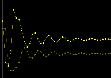
Figure 1. Oscillations of the host and parasitoid with increasing generations decaying to fixed values.
Click on the image to load it into your local Phaser.

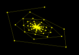
Figure 2: Asymptotically stable fixed point: It is often advantageous to plot the host against the parasitoid and construct phase portraits of the MAP as a dynamical system. For the same parameter values as in Figure 1, the host against the parasitoid are plotted. Notice that the orbit approaches an asymptotically stable fixed point.

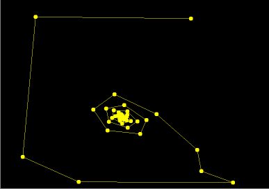
Figure 2. Asymptotically stable fixed point.

Figure 3: Poincare-Andronov-Hopf Bifurcation: For fixed r = 1.8, as the parameter a is increased the asymptotically stable fixed point loses its stability and gives rise to an attracting closed invariant curve. The `radius' of the curve grows with increasing values of a. This is the Poincare-Andronov-Hopf bifurcation for MAPs. Biologically, this important bifurcation gives rise to sustained stable oscillations of the host and parasitoid populations; the amplitude of the oscillations grow with increasing a.

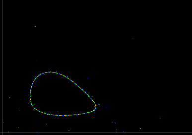
Figure 3. Poincare-Andronov-Hopf Bifurcation.

Figure 4: Invariant curve breaks up --- chaos: In this sequence of phase portraits, r =1.8 and a is varied far from the Poincare-Andronov-Hopf bifurcation value. As a is increased, the dynamics on the invariant curve exhibits intermittent periodic and quasi-periodic orbits (resonances). Eventually, the invariant curve loses its smoothness and breaks up into a chaotic attractor. The mathematical details of this sequence of events are rather complicated. Details of such an analysis for a different two-parameter planar map, Delayed Logistic MAP, are given in Aronson et al. [1982].

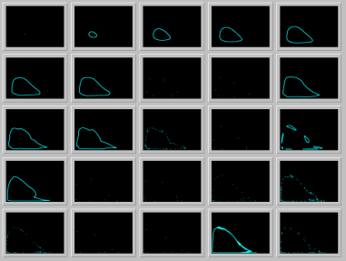
Figure 4. A sequence of phase portraits: r fixed, a varied.
Click on the image to load it into your local Phaser. To see a sequence of phase portraits, hit the "Slideshow" button on the button bar of the spawned Gallery, and Play.

Figure 5: Bifurcation diagram --- r fixed, a varied: To investigate further the dependence of the dynamics on the search efficiency parameter a, it is instructive to compute a bifurcation diagram of the map as seen below. Here the parameter r is fixed at r = 1.8, and a is increased from 0.2 to 1.7. The horizantal axis is the parameter a and the vertical axis is the host values.

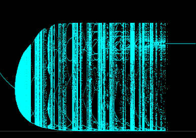
Figure 5. Bifurcation diagram: r fixed, a varied.

Figure 5: A sequence of bifurcation diagrams: It is not easy to visualize the dependence of a dynamical system on two parameters. One useful technique is to generate a sequence of bifurcation diagrams as seen below. Each bifurcation diagram is computed in a way similar to the one in Figure 6: for fixed r, a is varied from 0.2 to 1.7. For the bifurcation diagram in the first frame we set r = 2.0, and in the succeeding frames increase r by 0.01, eventually finishing with r = 2.08 in the last frame. Notice the sensitivity of the dynamics on the invariant closed curve.

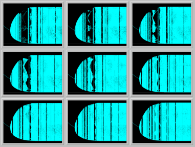
Figure 6. A sequence of bifurcation diagrams.
In each frame a is varied from a = 0.2 to a = 0.7, while r is advanced from r = 2.0 to r = 2.08 with increments of 0.01 in successive frames.

Experimental data:
We would appreciate receiving information about references on experimental data pertaining to the Beddington-Free-Lawton MAP.

Remarks:

The Beddington-Free-Lawton MAP succeeds in providing a quantitative possibility of bounded oscillations in host-parasitoid interactions. Perhaps, more significant implications of this model are highligted in the concluding paragraph of Beddington, Free, and Lawton [1975]:
"The existence of high periodic cycles or chaotic behaviour in predator-prey models (the distinction is unimportant for practical purposes) may be of considerable importance in interpreting the patterns of fluctuation shown by many arthropod populations in the field, as this implies the possibility of long term coexistence between predator and prey within well defined limits, but of a seemingly random nature. The temptation to ascribe such behaviour to `environmental fluctuations' is obvious. Thus a recognition that such behaviour may occur in an extremely simple, entirely deterministic predator-prey model is considerable importance."

Besides host density-dependence, there are other biological considerations that can stabilize the unbounded oscillations of the Nicholson-Bailey MAP. Based on experimental data, Hassell and Varley [1969] observed that the search efficiency parameter a in the Nicholson-Bailey MAP may not be constant but may decrease with increasing parasitoid density. The stabilizing effect of this assumption is demonstrated in the Suggested Explorations below.

Suggested Explorations:

Alone: Investigate numerically the fate of the host and the parasite in the absence of the other. For this purpose, set the initial density of the absent population to zero. Justify the results of your simulations from the model.

Stabiliy of the fixed point: Load Figure 2 into your local Phaser. By changing the parameter values a and r systematically, determine some ranges of the parameter values for which the positive fixed point remains asymptotically stable. Interpret your findings biologiccally.

Another fixed point: Verify that the origin is a fixed point. Investigate the stability type of this fixed point Discuss the ecological significance of your finding.

Bifurcation diagram for parasitoid: Load the Phaser Project in Figures 5. Keep the current settings, except that this time recompute the bifurcation diagram with the parasitoid values assigned to the vertical axis. Do you see any qualitative changes?

Impressive chaotic attractor: For the parameter values r = 2.55 and a = 0.5, there is an impressive chaotic attractor. To see it, click here.

Mutual interference: Besides the host density dependence, other considerations can also stabilize Nicholson-Bailey model. Hassell and Varley [1969] suggest that the search efficiency a may not be constant but may decrease with increasing parasitoid density. Indeed, based on laboratory experiments on parasitisation of a moth, Ephestia cantella, by an inchneumon, Nemeritis canescens, and other host-parasite systems, they proposed the formula
a = - QP_n^-m
for search efficiency, where Q and m are constants. By substituting this formula for a in the Nicholson-Bailey MAP they obtain Hassell-Varley MAP. Load this Phaser project and experiment with the values of the parameter m and discover its effect on stability. Laboratory experiments suggest 0.4-0.8 for the range of m. Further information about mutual interference can be found in Hassell [1978], [2000], and Maynard-Smith [1974].

Related modules:
Nicholson-Bailey MAP, Ricker MAP
References:

ARONSON, D.G., CHORY, M.A., HALL, G.R., and MCGEHEE, R. [1982]. "Bifurcations from an invariant circle for two-parameter families of the plane: a computer assisted study," Commun. Math. Phys., 83, 303-354.

BEDDINGTON, J.R., FREE, C.A., and LAWTON, J.H. [1975]. "Dynamic complexity in predator-prey models framed in difference equations," Nature, 255, 58-60.

HASSELL, M.P. and VARLEY, G.C. [1969]. "New inductive population model for insect parasites and its bearing on biological control," Nature, 223, 1133-7.

HASSELL, M.P. [1978]. The Dynamics of Arthropod Predator-Prey Systems. Princeton University Press

HASSELL, M.P. [2000]. The Spatial and Temporal Dynamics of Host-Parasitoid Interactions. Oxford University Press

MAYNARD-SMITH, J. [1968]. Mathematical Ideas in Biology. Cambridge University Press.
MAYNARD-SMITH, J. [1974]. Models in Ecology. Cambridge University Press.
Feedback:
Please write to us with your comments about this module.