Chapter 1: Stability of One-Dimensional Maps
Section 1.3: Maps vs. Differential Equations
-
- Example 1.2. Euler's Method.
Solving a differential on a computer requires a discretization of the continuous problem with a suitable method. The simplest such method is the Euler's Method. Below is a Phaser simulation of the differential equation
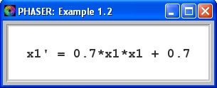 (1)
(1)
satisfying the initial value
x1(0) = 1.0 using Euler's Method with a step size of h = 0.1.
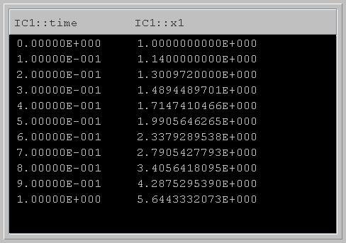
Figure 1.3.1. Euler approximation of Eq.(1) with step size of 0.1.In the figure below, the computed Euler approximation to the solution is plotted in Xi vs. Time view of Phaser.
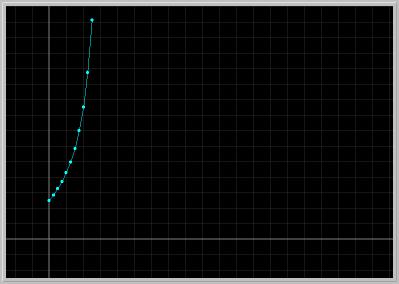
Figure 1.3.2. Euler approximation of Eq.(1) with step size of 0.1.Activities:
- Click on the first picture to load it into your local copy of Phaser.
- Now, we want to change the step size and observe its effect on the approximation. Following the instructions in (PhaserTip: Step Size) change the step size to 0.01. Clear and Go. Notice the new value of x1 at time 1 (the last line). Does it differ much from the value with step size of 0.1? Which value is more accurate?
- Click on the second picture to load it into your local copy of Phaser. Following the instructions in (PhaserTip: Step Size) change the step size to 0.01. Do not Clear; just hit Go button. Observe the difference between the old curve and the new one.
- Example 1.3: An Insect Population
A population of aphids can be modeled using a difference equation of the form
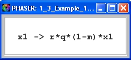 (2)
(2)
where
- x1 is the number of aphids,
- m is the fractional mortality in the young aphids,
- q is the number of progeny per female aphid,
- r is the ratio of female aphids to total adult aphids.
The asymptotic fate of the population is determined by the following conditions on the parameters:
- if rq(1 -m) < 1, then population goes extinct,
- if rq(1 -m) = 1, then population remains constant,
- if rq(1 -m) > 1, then population grows without bound.
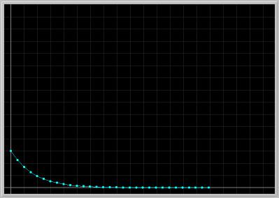
Figure 1.3.3. A decaying solution of Eq.(2). 30 generations of aphids are plotted for the initial number of x1 = 6 aphids, and the parameter values m = 0.9, q = 15, r = 0.5. Notice that the aphid population is moving towards extinction.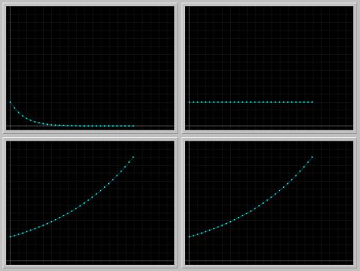
Figure 1.3.4. In the Phaser Gallery above, one decaying, one constant, and two growing solutions of the aphid population are shown.Activities:
- Click on the first picture to load it into your local copy of Phaser.
- Click the left mouse button while the cursor is anywhere along the vertical axis to mark a new initial condition. Clear and Go, and watch what happens to the solution as time goes on. Now, mark several initial conditions. Clear and Go. Do all solutions have the same fate?
- Click on the first picture again to reload it into your local copy of Phaser.
- Change the parameter q = 20 while keeping the other parameter values the same; Clear and Go. (PhaserTip: Changing Parameters) Do you get the frame in the upper right corner of the second picture?
- Without clicking, move your mouse cursor to one of the plotted points and determine its coordinates. (PhaserTip: Cursor Coordinates) Interpret this equilibrium value in terms of the current parameter values.
- Click on the second picture to load it into your local copy of Phaser.
- In the spawned Phaser Gallery, double click on any of the frames to load it into Phaser (Phaserize).
- Example 1.2. Euler's Method.
[ Previous Section | Next Section | Main Index | Phaser Tips ]