PHASER: Phaser Modules for Discrete Chaos

Modules: Discrete Chaos

Chapter 1: Stability of One-Dimensional Maps

Section 1.2: Maps Vs. Difference Equations

In this opening section, we showcase several striking Phaser simulations to spark your interest in the subject.

Example 1.1. The Logistic Map

The most famous one-dimensional map is, arguably, the Logistic MAP given by the formula

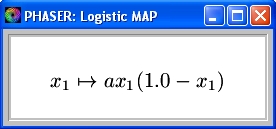
where a is a parameter in the range [1.0, 4.0]. We will study the dynamics and bifurcations of this map in detail later in the book.

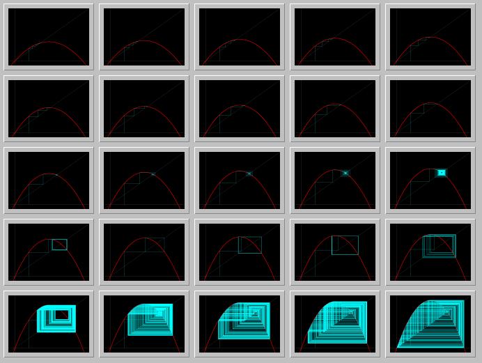
Figure 1.2.1 A Phaser Gallery of the Logistic MAP while the parameter a is incresed from 1.6 to 4.0.

Activities:

Click on the Gallery picture above to load it into your local copy of Phaser.
In the spawned Phaser Gallery window, click the Slideshow button on the button bar. Now a new Slideshow window should pop. On this window, click the Play button. Further information on Slideshow is available in (PhaserTip: Slideshow).

Example 1.2. The Sierpinski-Knopp (IFS) Map

Figure below is a Phaser Gallery of fractal curves with increasing dimension from 1 to 1.945 using Iterated Function Systems (IFS). We will see the mathematical details later; for now, just enjoy the show.

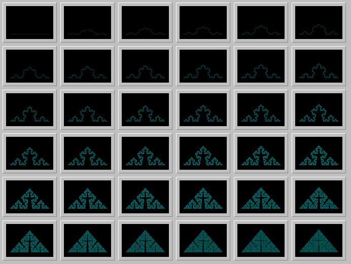
Figure 1.2.2. A Phaser Gallery of fractal curves with increasing dimension from 1 to 1.945 using Iterated Function Systems (IFS).

Activities:

Click on the Gallery picture above to load it into your local copy of Phaser.
In the spawned Phaser Gallery window, click the Slideshow button on the button bar. Now a new Slideshow window should pop. On this window, click the Play button. Further information on Slideshow is available in (PhaserTip: Slideshow).

Example 1.3. A 3-D Fractal Fern generated with IFS.
Figure below is a Phaser simulation of a three-dimensional picture of a fractal fern using Iterated Function Systems (IFS). We will see in Chapter 6 the mathematical details of creating interesting fractal images; for now, just enjoy the picture.

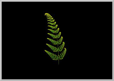
Figure 1.2.3. A 3-D fractal fern generated with IFS.

Activities:

Click on the picture above to load it into your local copy of Phaser.
You should see the picture of the fern computed and displayed in the large Phase Portrait view of Phaser. Position the cursor on or near the fern. While holding down the left mouse button you can rotate the fern by moving the mouse to see its 3D structure.
Notice the ``radio buttons'' on the lower right. Experiment with these buttons to control the rotations.
For more information on the IFS that is used to generate this picture, from the Equation menu select the nemu item View Current Equation Help.

| Next Section | Main Index | Phaser Tips ]