Chapter 1: The Stability of One-Dimensional Maps
Section 1.7: Criteria for Stability
-
- Example 1.10: Raphson-Newton's Method
In this example we will compute the square root of any positive number using the Newton-Raphson iteration. Consider the map of the form
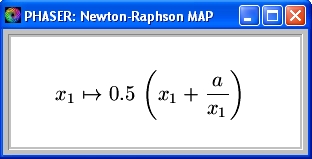 (1)
(1)
where a is a parameter. This map is the Newton-Raphson Map for finding the roots of x2 - a = 0. In the figure below, for a = 2, the graph of the map, 45-degree line and four solutions are plotted.
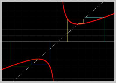
Figure 1.7.1. Newton-Raphson MAP in Eq.(1) for a = 2. Notice that there are two fixed points, the points of intersections of the graph and the 45-degree line. Both fixed points are asymptotically stable. Hence, iteration of any initial condition near a fixed point will approach the fixed point.Activities:
- Click on the picture to load it into your local copy of Phaser.
- Move your mouse cursor (without clicking) and determine the coordinates of the two fixed points. (PhaserTip: Cursor Coordinates)
- To get more precise digits of the fixed point, from the View menu select Xi Values and Go.
- You can also cycle through the Phaser views by clicking on the arrow buttons on the Phaser Button Bar. Now, using these arrows, return to 1-D Stair Stepper view. Set several more initial conditions by clicking the left mouse button near the fixed points. Clear and Go. (PhaserTip: Initial Conditions)
- Set the parameter to a = 3. (PhaserTip: Changing Parameters) Clear and Go. What happens to the fixed points?
- Example 1.11: A nonhyperbolic fixed point
In this example, we will examine the stability of the fixed point at the origin of the cubic MAP
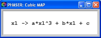 (2)
(2)
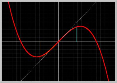
Figure 1.7.2. For a = -1, b = 1, and c = 0, the origin is a nonhyperbolic asymptotically stable fixed point.The two initial conditions in the picture above are iterated 50 times. Notice that the solutions are still far away from the origin. In numerical simulations it is important to be cognizant of the fact that approach to a nonhyperbolic asymptotically stable fixed point can be painfully slow. This fact has important consequences in following bifurcations in MAPs, as we shall see in later chapters.
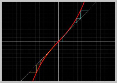
Figure 1.7.3. For a = 1, b = 1, and c = 0, the origin is a nonhyperbolic unstable fixed point.Activities:
- Click on the first picture to load it into your local copy of Phaser.
- Currently the Start Time = 0 and Stop Time = 50; thus the initial conditions are iterated 50 times. Set Stop Time to 100 (PhaserTip: Time). Clear and Go. Do the solutions get closer to the origin? Keep increasing the Stop Time so that visiually the orbits reach the origin.
- Set several more initial conditions by clicking the left mouse button near the fixed points. Clear and Go. (PhaserTip: Initial Conditions)
- Set the parameter to a = 0.5. (PhaserTip: Changing Parameters) Clear and Go. What happens to the number and the stability types of the fixed points?
- Change the values of the parameters a, b, c to investigate the dependence of the number and stability types of the fixed points on the coefficients of the cubic map. (PhaserTip: Changing Parameters)
- Example 1.10: Raphson-Newton's Method
Exercises:
-
18.
[ Previous Section | Next Section | Main Index | Phaser Tips ]