Chapter 1: The Stability of One-Dimensional Maps
Section 1.8: Periodic Points and their Stability
-
- Example 1.13: The Logistic II MAP
In this example we will investigate the periodic points of the quadratic map
 (1)
(1)
where a is a parameter. This quadratic map is equivalent to the usual form of the Logistic MAP by a change of variable. In the figure below, for a = 1, the graph of the map, 45-degree line and a solution starting near a fixed point are plotted.
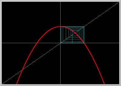
Figure 1.8.1. Logistic II MAP in Eq.(1) for a = 1. Note that the positive fixed point is unstable. A solution starting near this fixed point moves to an asymptotically stable periodic orbit of period 2 (the period-2 points are 0 and 1).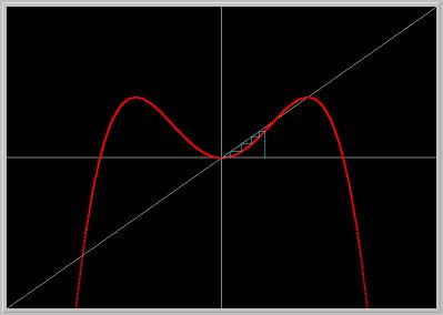
Figure 1.8.2. Second power of the Logistic II MAP in Eq.(1) for a = 1. The period-2 points 0 and 1 are two fixed points of second power of the map.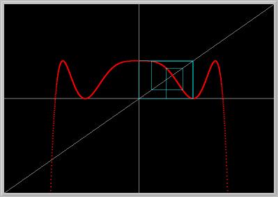
Figure 1.8.3. Third power of the Logistic II MAP in Eq.(1) for a = 1. Notice that there is only one fixed point which is the fixed point of the map itself as seen in the first figure above. Therefore, there is no period-3 orbit with minimal period 3.Activities:
- Click on the first picture to load it into your local copy of Phaser.
- Move your mouse cursor (without clicking) and determine the coordinates of the positive fixed point. (PhaserTip: Cursor Coordinates)
- To see where the orbit is going (omega-limit set) it is convenient to leave out transients. To accomplish this, Set the Start Time to 50. (PhaserTip: Time) Now the first 50 iterations of the initial conditions will be computed but not be plotted; iteratin 50-100 will be plotted. Clear and Go. You should see a rectangle whose corners at 0 and 1 (on the diagonal) are the period-2 points.
- Set the parameter to a = 1.3. (PhaserTip: Changing Parameters) Clear and Go. What happens to the period-2 points?
- Example 1.14: Periodic points of the Tent MAP
In this example, we will examine the piece-wise linear Tent MAP of the form
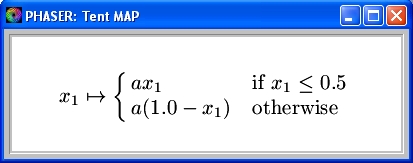
where a is a parameter. In the figures below, we set a = 2.
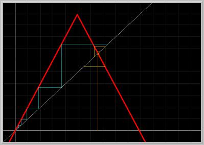
Figure 1.8.4. The graph of the Tent MAP for the parameter value a = 2.0, the 45-degree line, and two solutions (iterated 6 times) are plotted. The two fixed points are unstable. So, where do the two solutions go under further iterations?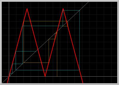
Figure 1.8.5. The second power of the Tent MAP. There is a periodic orbit of period-2, but it is unstable.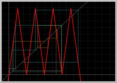
Figure 1.8.6. The third power of the Tent MAP. There are two periodic orbits of period-3, but they are unstable.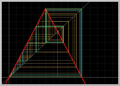
Figure 1.8.7. This is the same as the first picture of the Tent MAP except that now the two orbits are iterated further (59 times). Believe it or not, the orbits end up at the unstable fixed point at the origin; examine the numbers in the next figure.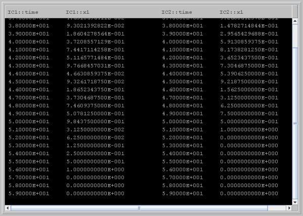
Figure 1.8.8. Note that after 59 iterations, the orbits end up at the unstable fixed point at the origin. This is a fantastic illustration of subtle difficulties associated with numerical computing, especially in chaotic systems. Mathematically, most orbits of the Tent MAP should be chaotic; indeed, the Tent MAP (for parameter a = 2) is mathematically equivalent to the Logistic MAP (a = 4) which is also chaotic. While the Logistic MAP displays chaotic behavior in numerical simulations, almost all orbits of the Tent MAP end up at the origin. Why? The answer lies in the binary architechure of the computer, and the fact that iteration under the Tent MAP amounts to shifting one bit to the left per iteration. Therefore, after about 60 iterations, all bits are shifted to zero. Amazing, is it not?Activities:
- Click on the first picture to load it into your local copy of Phaser.
- Hit the Numerics button to bring up the Numerics Editor. On the Numerics Editor, click the Current View button. Now click on the 1-D Stair Stepper on the control tree. Set Power of Map to Plot to 2 to plot the second power of the Tent MAP. Return to the main window, and Clear and Go. You should see the second picture.
- Using the instructions above, plot the third and fourth powers of the Tent MAP.
- Load the fourth picture by clicking on it. Click on the right arrow button on the button bar of the main window to bring up the Xi-Values view of Phaser. Hit Go; you should see the last picture. You can reach the same view from the View -> Xi-Values menu item.
- Click on the fourth picture again. Set the parameter to a = 1.9999. (PhaserTip: Changing Parameters) Set the Start Time = 400 and Stop Time = 1000; (PhaserTip: Time). Clear and Go. You should see a (non-periodic) chaotic orbit.
- Example 1.13: The Logistic II MAP
[ Previous Section | Next Section | Main Index | Phaser Tips ]