Chapter 1: The Stability of One-Dimensional Maps
Section 1.9: The Period-Doubling Route to Chaos
-
- Example: The Logistic MAP
In this example we will investigate the successive period doublings of periodic orbits of the Logistic MAP
 (1)
(1)
where a is a parameter. In the simulations below we will restrict the range of x1 to [0, 1] and the range of the parameter a to [1, 4].
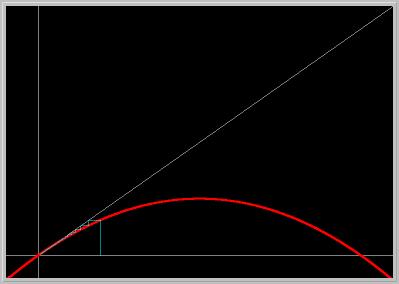
Figure 1.9.1. Logistic MAP in Eq.(1) for a = 1. The graph of the map, 45-degree line and a solution are plotted. Note that the (nonhyperbolic) fixed point at the origin is asymptotically stable.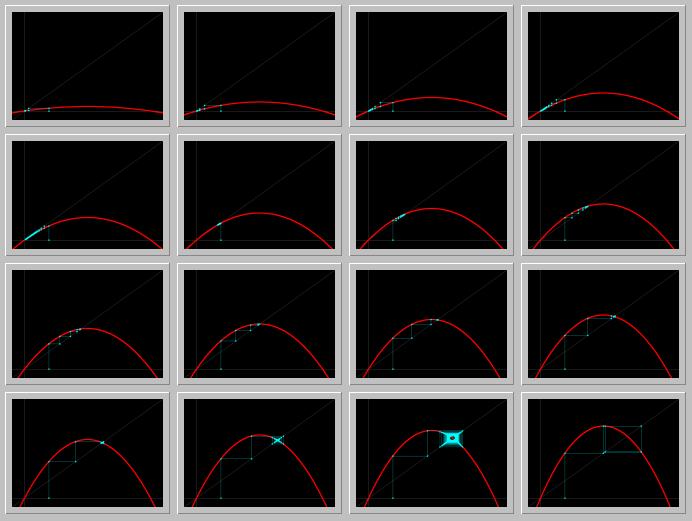
Figure 1.9.2. A Gallery of Logistic MAP in Eq.(1) as the parameter a is varied from 0.2 to 3.2 in increments of 0.2. Note that the fixed point at the origin becomes unstable by giving up its stability to another (positive) fixed point. As the parameter is increased further the positive fixed point becomes unstable and gives up its stability to a periodic orbit of period 2.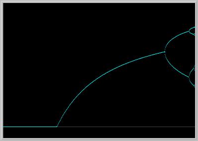
Figure 1.9.3. Bifurcation Diagram of the Logistic MAP in Eq.(1) while a is varied from 0 to 3.56. Notice that the fixed point at the origin gives up its stability to a positive fixed point. This fixed point gives up its stability to a periodic orbit of period 2. Three period-doubling bifurcations are visible in this diagram.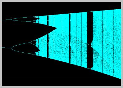
Figure 1.9.4. Bifurcation Diagram of the Logistic MAP in Eq.(1) while a is varied from 3.4 to 4.0.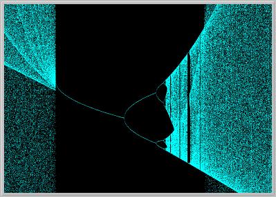
Figure 1.9.5. Bifurcation Diagram of the Logistic MAP in Eq.(1) while a is varied from 3.818604651162791 to 3.869767441860465. This is a blown-up version of a small window in the middle portion of the period-3 orbit in the previous bifurcation diagram.Activities:
- Click on the Gallery (second) picture to load it into your local copy of Phaser. Click the Slideshow button on the Gallery and hit play to see the slideshow. (PhaserTip: Slideshow)
- Click on the third picture (period doublings) to load it into your local copy of Phaser. Move your mouse cursor (without clicking) and determine the values of a at which the period-doubling bifurcations are happening. (PhaserTip Cursor Coordinates)
- Click on the fourth picture to load it into your local copy of Phaser. Set several more initial conditions by clicking the left mouse button. Clear and Go. (PhaserTip: Initial Conditions) Now, the bifurcation diagram will be computed several times using different initial conditions. Note that the bifurcation diagram seems to be independent of (most) initial conditons.
- Click on the last picture to load it into your local copy of Phaser. Notice ZOOM in the center of the Tool bar. Mouse is used for several different purposes such as selecting initial conditions or zooming into a selected region of a view. The current state of mouse is indicated in the drop down widget in the center of Tool bar. So, now click the left mouse button at a point on the bifurcation diagram and while holding down the mouse button, select a rectangle and let the mouse button go. You should the selected region of the bifurcation amplified. Try it.
- Example 1.14: Bifurcation diagram of the Tent MAP
In this example, we will view the bifurcation diagram of the piece-wise linear Tent MAP of the form
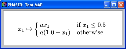
where a is a parameter.
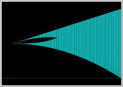
Figure 1.9.6. Bifurcation diagram of the Tent MAP while the parameter a is varied from 0.9 to 2.Activities:
- Click on the picture to load it into your local copy of Phaser.
- Notice that the current mouse function is IC for Initial Conditions as indicated in the center of the Tool Bar. From this drop-down widget, select ZOOM. Then as described in the Activities above, explore the details of the bifurcation diagram by zooming into selected regions.
- Example: The Logistic MAP
[ Previous Section | Next Section | Main Index | Phaser Tips ]