Chapter 1: Stability of One-Dimensional Maps
Section 1.4: Linear Maps/Difference Equations
-
- Linear Maps:
Linear Maps of the form
 (1)
(1)
where a and b are parameters are central in the theory and applications of Maps. Below we will see Phaser simulations of this map for various values of the parameters a and b. For simplicity, we will fix b = 0 and vary a. Here are some key observations:
- if a < 0 then solutions alternate from positive to negative, or vice versa,
- if a ≥ 0 then solutions keep the same sign,
- if |a| < 1 then all solutions approach the unique fixed point at the origin,
- if |a| > 1 then al solutions, except the origin, run away from the origin without bound; that is, the fixed point at the origin is unstable,
- if a = -1 then all solutions oscillate with period 2,
- if a = 1 then all solutions are fixed points.
Now, let us see Phaser simulations of some of these cases:
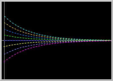
Figure 1.4.1. Linear MAP: a = 0.9, b = 0. The origin is an asymptotically stable fixed point (monotone approach).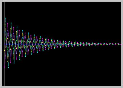
Figure 1.4.2. Linear MAP: a = -0.9, b = 0. The origin is an asymptotically stable fixed point (oscillatory approach).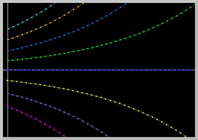
Figure 1.4.3. Linear MAP: a = 1.05, b = 0. The origin is an unstable fixed point.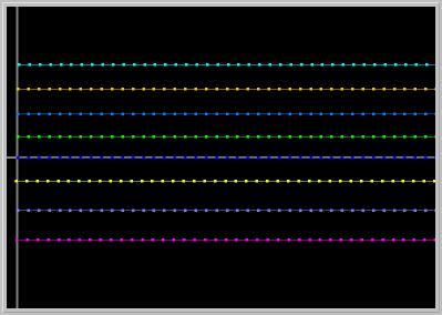
Figure 1.4.4. Linear MAP: a = 1, b = 0. The origin is a stable fixed point (all points are fixed).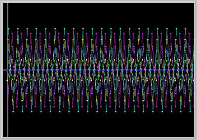
Figure 1.4.5. Linear MAP: a = -1, b = 0. The origin is a stable fixed point (all solutions are periodic with period 2).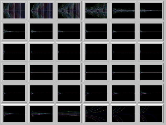
Figure 1.4.5. A Gallery of solutions of Linear MAP (1) while b = 0 fixed and a is varied from a = -1.25 to a = 1.20 with increments of 0.07.Activities:
- Click on the first picture to load it into your local copy of Phaser.
- Change the parameter b = 0.2. (PhaserTip: Changing Parameters) Clear and Go. Do you notice any qualitative or quantitative change in the picture?
- Repeat the parameter change above with the next three pictures.
- Click on the Gallery picture to load it into your local copy of Phaser.
- In the spawned Phaser Gallery window, click the Slideshow button on the button bar. Now a new Slideshow window should pop. On this window, click the Play button. Further information on Slideshow is available in (PhaserTip: Slideshow).
- Example 1.4: Administering a drug
Suppose that a drug is administered according to the formula
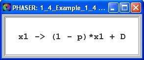 (2)
(2)
where
- x1 is the amount of drug,
- p is the fractional of drug that has been eliminated from the body,
- D is the new dose of the drug.
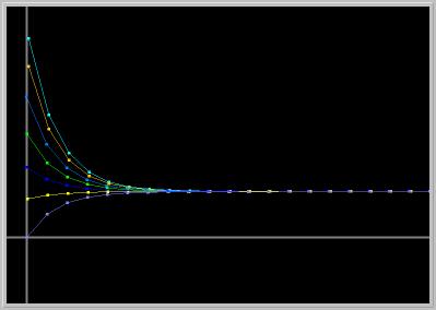
Figure 1.4.6. All solutions of Eq.(2) approaching the same steady state. Twenty days of the drug amount are plotted for various initial amounts of drug x1, and the parameter values p = 0.5 and D = 0.7. Notice that the amount of drug is approaching a constant value regardless of the initial amount.Activities:
- Click on the picture to load it into your local copy of Phaser.
- Without clicking, move your mouse cursor to the steady state value and determine its vertical coordinate. (PhaserTip: Cursor Coordinates) Is the steady state (fixed point) value approximately D/p?
- Experiment with several values of the parameters p and D (PhaserTip: Changing Parameters) Note any qualitative or quantitative changes in the pictures. For fixed parameter values, does the steady state depend on the initial condition?
- Linear Maps:
Exercises:
-
3.
[ Previous Section | Next Section | Main Index | Phaser Tips ]