Newton's first differential equation
Highlights:
 Historical:
"But this will appear plainer by an Example or two. ..."
(Newton
1671) --- After outlining his general method for finding solutions
of differential equations. The equation in this module is his first
significant example.
Historical:
"But this will appear plainer by an Example or two. ..."
(Newton
1671) --- After outlining his general method for finding solutions
of differential equations. The equation in this module is his first
significant example.
Mathematical: Newton obtained the solution of a differential equation satisfying a given initial condition in terms of infinite series. At each stage of his series solution, he inserted the series into his differential equation and integrated the resulting polynomial.
Prerequisites:
Linear ODEs
Equation:
y˙ ⁄ x˙ = 1 - 3x + y + x x + x y
Quantities:
| x | : "the Correlate Quantity" |
| y | : "the Relate Quantity" |
| x˙ | : "the Fluxion of x" |
| y˙ | : "the Fluxion of y" |
Discussion:
Newton's book,
ANALYSIS Per Quantitatum, SERIES, FLUXIONES,
AC DIFFERENTIAS: cum Enumeratione Linearum
TERTII ORDINIS,
consists of one dozen problems.
His second problem
"PROB. II An Equation is being proposed, including the Fluxions of Quantities, to find the Relations of those Quantities to one another"
is devoted to a general method of finding the solution of an initial-value problem for a scalar differential equation in terms of infinite series. The equation above is his first significant example in this section.
Newton thought of Mathematical quantities as being generated by a continuous motion. He called such a flowing quantity a fluent (variable), and referred to its rate of change as the fluxion of fluent of the quantity and denoted it by a dot over the quantity. He denoted the change of Relate Quantity (dependent variable) with respect to the Correlate Quantity (independent variable) with the ratio of their fluxions. If we reinterpret Newton in our current calculus jargon as x˙ = dx/dt, y˙ = dy/dt, and y˙ ⁄ x˙ = dy/dx, then Newton's differential equation becomes dy/dx = 1 - 3x + y + x2 + x y.
Newton's Solution:
Now, we will paraphrase Newton's steps and obtain several terms of his power series
solution y(x) of his differential equation satisfying the initial
condition y(0) = 0. Start with the first term
y = 0 + …
and insert it into the differential equation to obtain
y′ = 1 + … .
Now, integrate this with respect to x,
y = x + …
to obtain the next term in the series. Inserting this series for y into
the differential equation, yields
y′ = 1 - 2x + …
integration of which gives
y = x - x2 + … .
The next iteration of this process gives
y′ = 1 - 2x + x2 + …
and
y = x - x2 + (1/3)x3 + … .
Newton continues several more iterations and arrives at the solution
y = x - x2 + (1/3)x3 - (1/6)x4 +
(1/30)x5 - (1/45)x6 + … .
Newton's Demonstration: It is prudent to verify that a proposed solution of a differential equation indeed satisfies the differential equation. Here is how Newton demonstrates the validity of his solution:
DEMONSTRATION"56. And thus we have solved the Problem, but the demonstration is still behind. And in so great a variety of matters, that we may not derive it synthetically, and with too great perplexity, from its genuine foundations, it may be sufficient to point it out thus in short, by way of Analysis. That is, when any Equation is propos'd, after you have finish'd the work, you may try whether from the derived Equation you can return back to the Equation propos'd ... And thus from y˙ = 1 - 3x + y + x x + x y is derived y = x - x2 + (1/3)x3 - (1/6)x4 + (1/30)x5 - (1/45)x6 , &c. And thence by Prob. I. y˙ = 1 - 2x + x2 - (2/3)x3 + (1/6)x4 - (2/15)x5 , &c. Which two values of y˙ agree with each other, as appears by substituting x - xx + (1/3)x3 - (1/6)x4 + (1/30)x5 , &c. instead of y in the first value."
Dynamics:
A series solution of an initial-value problem, in principle, should yield better approximations to the solution as more terms of the series are included. In Figure 1., third through sixth-order approximations of the Newton's series solution are plotted.
Phaser simulation:
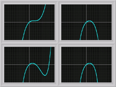
Figure 1. Third through sixth order series approximations of the solution of Newton's differential equation.
Click on the picture to load it into your local Phaser.
In Figure 2., the actual solution of Newton ODE satisfying the initial condition y(0) = 0 is plotted in blue. The additional solution in yellow satisfies the initial condition y(0) = 1; Newton's series of this solution is given in the Suggested Explorations below.
Phaser simulation:
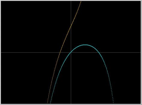
Figure 2. Two solutions of Newton's differential equation.
Click on the picture to load it into your local Phaser.
It was indicated above that one can expect better approximations as more terms of the series are included. However, this expectation holds only locally near the initial condition, but not globally. Indeed, the fourth-order approximation appears to be more faithful to the actual solution than the fifth-order approximation.
Mathematical results:
Newton ODE is a scalar linear differential equation for which there exists a formula for the solutions. Full details of the use of this formula for Newton ODE is available in a PDF file. You will notice in this file, however, that one of the requisite integrations involves the error function which cannot be expressed in terms of elementary functions.
Suggested Explorations:
y = 1 + 2x + x3 + (1/4)x4 + (1/4)x5 + … .
Demonstrate the validity of Newton's solution a la Newton. This solution is plotted in yellow in Figure 2 above.
y = a + x + ax - xx + axx + (1/3)x3 + (2/3)ax3 + …
which being found, you may substitute 1, 2, 0, (1/2), or any other number, and thereby obtain the Relation between x and y an infinite variety of ways."
In other words, Newton computed the solution of his equation for the initial condition y(0) = a. Verify his answer.
"32. And after the same manner the Equation y˙ ⁄ x˙ = 3y - 2x + x/y - 2y/(xx) being proposed; if, by reason of the Terms x/y and 2y/(xx), I write 1 - y for y, 1-x for x, there will arise y˙ ⁄ x˙ = 1 - 3y + 2x + (1-x)/(1-y) + (2y -2)/(1 - 2x + x2). But the Term (1 - x)/(1 - y) by infinite Division gives 1 - x + y - xy + y2 - xy2 + y3 - xy3, &c. and the Term (2y - 2)/(1 -2x + xx) by a like Division gives 2y - 2 + 4xy - 4x + 6x2y - 6x2 + 8x3y - 8x3 + 10x4y -10x4, &c. Therefore y˙ ⁄ x˙ = -3x + 3xy + y2 - xy2 + y3 - xy3, &c. + 6x2y - 6x2 + 8x3y - 8x3 + 10x4y - 10x4, &c.Perform the "infinite Divisions" and verify Newton's calculations.
Related modules:
None.References:
HAIRER, E., NORSETT, S., and WANNER [1987]. Solving Ordinary Differential Equations. Springer-Verlag, New York.
NEWTON, I. [1736]. The Method of Fluxions and Infinite Series; with its Applications to the Geometry of Curve-lines by the Inventor Sir Isaac Newton, Kt., Late President of the Royal Society. / Translated from the Author's Latin Original not yet made publick. / To which is subjoin'd, A perpetual Comment upon the whole Work, Consisting of Annotations, Illustrations, and Supplements, In Order to make this Treatise A Compleat Institution for the use of Learners. / By John Colson. London: Printed by Henry Woodfall; And Sold by John Nourse, at the Lamb without Temple-Bar. M.DCCXXVI.
O'CONNOR, J.J. and ROBERTSON, E.F. Sir Isaac Newton:
http://www-gap.dcs.st-and.ac.uk/~history/Mathematicians/Newton.htmlPrintable Document:
An expanded and printable version of this module in PDF format is available at:
http://www.phaser.com/modules/historic/newton/isaac_newton_ode.pdfFeedback:
Please write to us with your comments on this module.